Half Moons Example

This notebook demonstrates the use of Shadow for the canonical semi-supervised learning example: half moons.

A strictly supervised (only labeled data) baseline model is trained alongside the same model architecture trained using Exponential Averaging Adversarial Training (EAAT).

import shadow.utils
shadow.utils.set_seed(0, cudnn_deterministic=True)  # set seeds for reproducibility

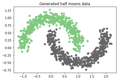
Create Data

Half moons data is generated using the scikit-learn toy datasets interface.

%matplotlib inline
import matplotlib.pyplot as plt
from sklearn import datasets

n_samples = 1000  # number of samples to generate
noise = 0.1  # noise to add to sample locations
x, y = datasets.make_moons(n_samples=n_samples, noise=noise)

plt.scatter(*x.T, c=y, cmap=plt.cm.Accent)
plt.title("Generated half moons data");

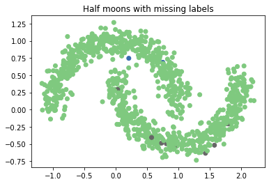
Drop Labels

Since the half moons dataset is synthetic, all labels are available. To test out the semi-supervised learning infrastructure, we artificially remove 99% of labels. To demarcate “unlabeled” samples, we set their corresponding label to -1. This is convenient method to handle missing classification labels in torch, as we will see later in the definition of the cross entropy loss.

import copy
import numpy as np

unlabeled_frac = 0.99  # fraction of data to drop labels

y_ssml = y.copy()
unlabeled = np.random.choice(range(n_samples), size=int(unlabeled_frac * n_samples), replace=False)
y_ssml[unlabeled] = -1  # set missing labels to -1

plt.scatter(*x.T, c=y_ssml, cmap=plt.cm.Accent)
plt.title("Half moons with missing labels");

Train a classifier

Next, we will instantiate the various training objects used in torch: models, optimizers, and criterion.

Model Architecture

We define our simple model architecture for use on this toy problem. We wrap this model into a factory, so that we can produce it twice: once for the baseline and once for the semi-supervised test.

import torch

def model_factory():
    return torch.nn.Sequential(
        torch.nn.Linear(2, 10),
        torch.nn.ReLU(),
        torch.nn.Linear(10, 10),
        torch.nn.ReLU(),
        torch.nn.Linear(10, 2)
    )

device = torch.device('cpu')  # run on cpu, since model and data are very small

Baseline Model

The baseline model and optimizer are defined normally.

bl = model_factory().to(device)
bl_opt = torch.optim.SGD(bl.parameters(), lr=0.1, momentum=0.9)

Semi-supervised Model

The semi-supervised model is instantiated with one critical difference: the model is wrapped by the shadow-provided ssml technique (in this case Exponential Averaging Adversarial Training). The wrapper defines additional technique-specific hyperparameters, but should be instead of using a plain model directly.

import shadow.eaat
eaat = shadow.eaat.EAAT(model=model_factory(), alpha=0.8, xi=1e-4, eps=0.3).to(device)
eaat_opt = torch.optim.SGD(eaat.parameters(), lr=0.1, momentum=0.9)

Loss function

As was alluded to earlier, using -1 to indicate missing labels is convenient in torch. That is because our standard CrossEntropyLoss criterion already has a parameter to ignore specific label values. We simple instatiate the loss function as normal, but set that parameter (ignore_index) to our unlabeled value.

Other loss functions may provide such a functionality or may need to be manually modified so as to mask data with missing labels.

xEnt = torch.nn.CrossEntropyLoss(ignore_index=-1).to(device)

Training Loop

We train both the baseline and semi-supervised models at the same time using standard torch conventions. Since the half-moons dataset is a small toy example, we use the whole dataset at once instead of batching.

The only modification to the training loop needed for the semi-supervised model is that the loss function is composed of both the supervised loss (xEnt) as well as a technique provided unsupervised loss (eaat.get_technique_cost). The details of this unsupervised loss vary between techniques, but it provides the mechanism for semi-supervised learning.

n_epochs = 500
xt, yt = torch.Tensor(x).to(device), torch.LongTensor(y_ssml).to(device)
for epoch in range(n_epochs):
    # Standard forward/backward pass for training baseline
    out = bl(xt)
    loss = xEnt(out, yt)  # ignores the unlabeled data (-1)
    bl_opt.zero_grad()
    loss.backward()
    bl_opt.step()

    # Forward/backward pass for training semi-supervised model
    out = eaat(xt)
    loss = xEnt(out, yt) + eaat.get_technique_cost(xt)  # supervised + unsupervised loss
    eaat_opt.zero_grad()
    loss.backward()
    eaat_opt.step()

Evaluate performance

Finally, we evaluate and compare performance between our strictly supervised baseline model, and the same model trained using semi-supervised learning.

It is critical to set the EAAT wrapped model into eval mode after training, so as to disable certain augmentations performed for semi-supervised learning.

bl.eval()
eaat.eval();

The accuracy provided by SSML greatly outperforms that of the baseline, as we would expect.

import shadow.losses

bl_pred = torch.max(bl(xt), 1)[-1]
eaat_pred = torch.max(eaat(xt), 1)[-1]

print("bl accuracy:", shadow.losses.accuracy(bl_pred, torch.LongTensor(y)).data)
print("eaat accuracy", shadow.losses.accuracy(eaat_pred, torch.LongTensor(y)).data)

bl accuracy: tensor(75.9000, dtype=torch.float64)
eaat accuracy tensor(98.7000, dtype=torch.float64)

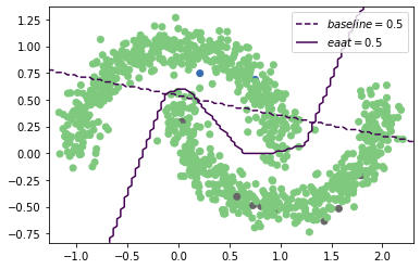
Visualize Decision Boundary

In order to get a better sense of how “good” our EAAT trained model is, we can leverage the fact that half-moons is a toy 2D dataset to visualize the model decision boundary. We define a 2D meshgrid over the data space and evaluate the models over the grid. We then plot the contour corresponding to a score of 0.5, which represents the decision boundary.

As illustrated in the plot, the baseline learns exactly what it can from the labeled data. However the semi-supervised trained model learns both labeled and unlabeled data and captures the overall data trends despite having labels for only 1% of the training data.

# Determine grid range
x0_min, x0_max = x[:, 0].min() - 0.1, x[:, 0].max() + 0.1
x1_min, x1_max = x[:, 1].min() - 0.1, x[:, 1].max() + 0.1

# Create grid
x0, x1 = np.meshgrid(np.linspace(x0_min, x0_max, 100),
                     np.linspace(x1_min, x1_max, 100))
grid = torch.FloatTensor(np.hstack((x0.reshape(-1, 1), x1.reshape(-1, 1))))

# Plot the data
plt.scatter(*x.T, c=y_ssml, cmap=plt.cm.Accent)

# Evaluate baseline on the grid and plot decision boundary
bl_pred = torch.max(bl(grid), 1)[-1].numpy().reshape(x0.shape)
cs = plt.contour(x0, x1, bl_pred, levels=[0.5], linestyles='--')
h1, l1 = cs.legend_elements("baseline")

# Evaluate EAAT on the grid and plot decision boundary
eaat_pred = torch.max(eaat(grid), 1)[-1].numpy().reshape(x0.shape)
cs = plt.contour(x0, x1, eaat_pred, levels=[0.5])
h2, l2 = cs.legend_elements("eaat")

plt.legend(h1 + h2, l1 + l2)

<matplotlib.legend.Legend at 0x7f09007b5e20>