Overview
The shadow python package implements multiple techniques for semi-supervised learning.
Semi-supervised learning (SSL) enables training a model from both labeled and unlabeled data, and is typically
used in contexts in which labels are expensive to obtain but unlabeled examples are plentiful.
This is illustrated in Fig. 1.
This package is built upon the PyTorch machine learning framework.
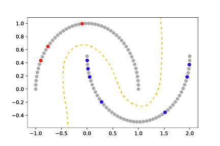
Fig. 1 Semi-supervised learning uses both labeled (red and blue) and unlabeled (grey) data to learn a better model (gold dashed line).
Package Design
Semi-supervised techniques require two steps for integration into an existing supervised workflow. First, the existing PyTorch model is wrapped using the desired technique, in this case Exponential Average Adversarial Training (EAAT):
model = ...  # PyTorch torch.nn.Module
eaat = shadow.eaat.Eaat(model)  # Wrapped model
Next, the loss function computation during training is modified to include a call to the wrapper-provided get_technique_cost:
loss = criterion(x, y) + eaat.get_technique_cost(x)
Note that as posed in this code example, both labeled and unlabeled data are passed to the supervised part of the loss function, criterion. The PyTorch CrossEntropyLoss provides an ignore_index parameter. For samples without labels, y is set to this ignore_index. Other loss functions can be modified to mask the mini-batch accordingly.
Consistency Regularization
Semi-supervised learning requires assumptions about the underlying data in order to make use of the
unlabeled data. The majority of techniques implemented in the shadow package are consistency
regularizers: they assume that the target variable changes smoothly over the data space. Said
another way: data points close to each other likely share the same label. To enforce this smoothness,
a consistency penalty is added to the overall loss function as:
where \(\mathcal{L}\) is the original loss function, \((x_l, y_l)\) represents labeled data, \(f_\theta(x_l)\) represents the predictions from model \(f_\theta\), \(\alpha\) represents a relative penalty weighting (hyperparameter), \(g\) represents a consistency enforcing function, and \(x\) represents all data (labeled and unlabeled). Critically, the consistency function depends upon input data but not the labels, which enables semi-supervised learning. The specific form of \(g\) and the mechanism by which it enforces consistency varies between techniques.
Virtual Adversarial Training
Virtual Adversarial Training [Miyato18] (VAT) enforces model consistency over small perturbations to the input. Accordingly, the consistency term penalizes the difference between the model output of the data and the model output of perturbed data:
where \(d\) represents some divergence function (typically mean squared error or Kullback-Liebler divergence) and \(r_{adv}\) represents a small data perturbation. Instead of sampling perturbations \(r_{adv}\) at random, VAT generates perturbations in the virtual adversarial direction which corresponds to the direction of greatest change in model output, enabling more effective regularization. This is illustrated in Fig. 2.
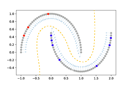
Fig. 2 Virtual Adverarial Training [Miyato18] enforces consistency over perturbations to model input (shown as arrows). Pertubations are in the virtual adversarial direction, which represents the maximum change in model output.
Mean Teacher
Mean Teacher [Tarvainen17] (MT) enforces consistency over model weights. MT builds on the idea that averaging over training epochs (temporal ensembling) produces more stable predictions. While temporal ensembling originally averaged the output values, [Tarvainen17] demonstrated advantages and performance increases by using the exponential moving average (EMA) of the model weights (denoted as the “teacher”) during training. Additionally, MT further assumes that additive noise or realistic data augmentation should minimally affect current model predictions. The consistency loss term for Mean Teacher is therefore:
Where \(f_\theta'\) (teacher) represents the weight-wise exponential moving average of the model \(f_\theta\) (student), and \(n\) represents additive noise. This is illustrated in Fig. 3.
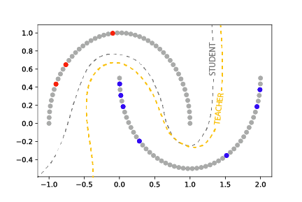
Fig. 3 Mean Teacher [Tarvainen17] enforces consistency over model weights between a student (grey dashed line) and a teacher (gold dashed line) model. The teacher model is the weight-wise exponential moving average during training of the student.
Exponential Averaging Adversarial Training
A natural extension of MT and VAT is to leverage the MT teacher-student framework but utilize virtual adversarial perturbations to regularize the student. We denote this joint implementation as Exponential Average Adversarial Training [Linville21] (EAAT). The consistency function is given as:
This is illustrated in Fig. 4.
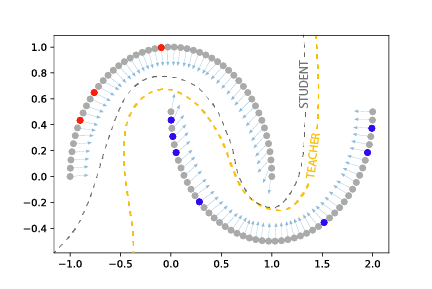
Fig. 4 Exponential Averaging Adversarial Training [Linville21] combines both VAT and MT by enforcing consistency between a teacher and a student in which the student is given virtual adversarial perturbed data.
Practical Recommendations
The techniques in shadow were developed to test the performance of
various approaches to semi-supervised learning in a new application domain: seismic
waveform data. Although we primarily focus on classification, the
generalized framework provided here supports both classification and
regression tasks. Although all new datasets and techniques require significant investment in
tuning and optimization, for many of these SSL techniques we have
observed significant sensitivity to small changes in hyperparameter settings
and experiment set-up. Below, we offer some lessons learned for training and experiment setup
for these techniques.
Although VAT and EAAT seem to tolerate significant imbalance between unlabeled and labeled data fractions per class, MT often learns best with a 50/50 labeled/unlabeled data fraction within each mini-batch. In the case of small label budgets this implies significant oversampling of labeled data. In many of our experiments, we found a consistency cost weighted at 2-4 times that of the class loss enabled meaningful learning beyond simply fitting the label set.
For example, to weight the consistency cost:
loss = criterion(x, y) + weight * mt.get_technique_cost(x)
VAT, on the other hand, often trains longer under large label/unlabeled fractions per batch, can tolerate a range of loss weights, but can be sensitive to the perturbation amplitude (xi). We suggest xi be tuned in advance of model training for new datasets to ensure the perturbation amplitudes are not unreasonably large or converge to zero over one power iteration. The xi_check parameter can be turned on to guide initial order of magnitude studies in this regard. Likewise, the eigenvector estimation used to find virtual adversarial directions yields a sign ambiguity: perturbations are often estimated in the negative of the direction that provides the maximum change in model output. We provide a method to resolve the direction ambiguity as a technique parameter: flip_correction (defaults to True). If set to False, computation is faster but convergence may be slower as competing directions may more closely resemble random perturbations.
EAAT has more complexity than MT or VAT alone; it requires consistency between input and adversarially perturbed input on the exponential average model. Added loss complexity often requires more extensive hyperparameter exploration. In our experiments, this included the considerations mentioned above for both MT and VAT and model depth, which appeared to limit SSL performance more than fully-supervised learning in the same data regime using EAAT.
In [Linville21], we examine the performance between MT, VAT, and EAAT against several baselines in a label-limited regime (where unlabeled data significantly outweighs the labeled data quantity). In these experiments, SSL outperforms baselines significantly. However, we also highlight that there is a limit to SSL performance as the number of available labels increases. When larger label fractions are available, SSL for our data can typically match but not increase performance compared to fully-supervised models, but at the expense of significantly more time spent on parameter optimization. One exception is that adding even minimal quantities of unlabeled data from out-of-domain (OOD) examples, in this case geographically, can positively impact prediction accuracy on new OOD examples, even when the number of unlabeled OOD examples is small compared to the number of labeled examples.
We hope the consistency-based SSL techniques provided here enable exploration on a wide variety of problems and datasets. To get you started, we provide a simple use example on MNIST available in MNIST Example.